State of Australia’s Marine Microbial Communities:2019

Author: Martin Ostrowski

Contact: martin.ostrowski@uts.edu.au

This is an R notebook providing details of the data and code for the analyses presented in the State and Trends Report for Australia’s Oceans and seas. The examples set out here provide a guide for accessing the processed Bacterial 16S data from the Australian Microbiome Initiative portal and observing the relative abundance of microbial taxa at different taxonomic levels.

Load the contextual data and plot a map and time series of the samples collected for ‘pelagic’ and ‘coastal’ datasets
Load the processed amplicon table
Plot alpha and beta-diversity for the National Reference Station Time Series
Time series plots for specific taxonomic ranks

Load the package libraries

library(tidyverse)
library(oce) #

1. Load the contextual metadata and streamline some formatting. (This will make things easier later)

contextual.long <- read_csv('~/MarineMicrobes Dropbox/uniques/BRT_2019/input/contextual_marine_201907.csv')

colnames(contextual.long) <- gsub(" ", "_", colnames(contextual.long), fixed = TRUE) #remove spaces
colnames(contextual.long) <- gsub("[", "", colnames(contextual.long), fixed = TRUE) #remove brackets
colnames(contextual.long) <- gsub("]", "", colnames(contextual.long), fixed = TRUE)
colnames(contextual.long) <- gsub("/", "_per_", colnames(contextual.long), fixed = TRUE)
colnames(contextual.long) <- tolower(colnames(contextual.long)) #all lowercase

contextual.long <- contextual.long  %>%
  separate (sample_id, c("num", "code"), sep='/')

2. Taming the factors in the contextual data

Factors help us organise the data by keeping things in the order we prefer and allowing us to subset according to our interests. Some effort here will keep things manageable.

Several factors can be split, for example, by separating the YYYY-MM-DD format date into year, month and day.

Add levels for the newly created months so they appear in the correct order (otherwise they are ordered alphabetically).

Convert some flagged data points in the nutrient data to NAs

contextual.long <- contextual.long %>%
    separate(date_sampled, c('year','month','day'), sep='-', remove=F) 

contextual.long$month.abb <- factor(month.abb[as.integer(contextual.long$month)], 
    levels=c(month.abb[seq(1,12,1)])) 

contextual.long$nitrate_nitrite_μmol_per_l[contextual.long$nitrate_nitrite_μmol_per_l == -999.000]<-NA;
contextual.long$phosphate_μmol_per_l[contextual.long$phosphate_μmol_per_l == -999.000]<-NA;
contextual.long$salinity_ctd_psu[contextual.long$salinity_ctd_psu == -999.000]<-NA;
contextual.long$silicate_μmol_per_l[contextual.long$silicate_μmol_per_l == -999.0000]<-NA;
contextual.long<- contextual.long[contextual.long$salinity_ctd_psu > 2,]

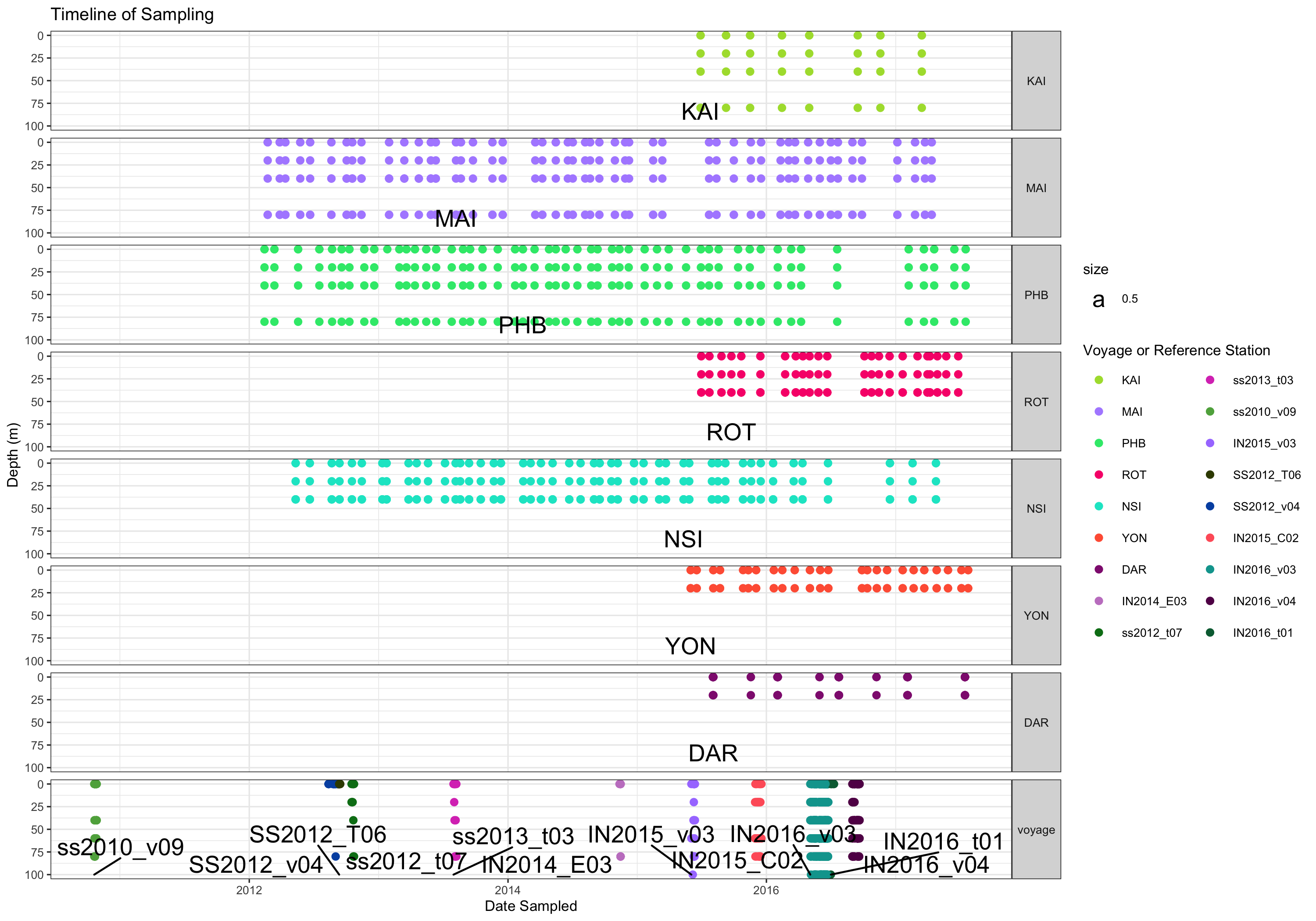
To examine the extent of the data in time and space plot the sites where the the samples have been collected from and a timeline of sample collection. Some more effort with factors now will help us do things more efficiently later. We’ll get to the goos stuff soon.

contextual.long$nrs_location_code_voyage_code <- factor(contextual.long$nrs_location_code_voyage_code, levels=c("KAI","MAI","PHB","ROT","NSI","YON","DAR","IN2014_E03","ss2012_t07","ss2013_t03","ss2010_v09","IN2015_v03","SS2012_T06","SS2012_v04", "IN2015_C02", "IN2016_v03", "IN2016_v04", "IN2016_t01"))

contextual.long$type <-contextual.long$nrs_location_code_voyage_code
contextual.long$type<-fct_expand(contextual.long$type, "voyage")

contextual.long$type[!contextual.long$type %in% c("KAI","MAI","PHB","ROT","NSI","YON","DAR")]<- "voyage"
contextual.long$type<-factor(contextual.long$type, levels=c("KAI","MAI","PHB","ROT","NSI","YON","DAR", "voyage"))

sites<- contextual.long[!duplicated(contextual.long$nrs_location_code_voyage_code),]

sitecols<-c("#abdd3a","#b08eff","#2fe879","#f81f79","#00e6cc","#ff6143","#90217f","#c583c9","#007c1a",
            "#da40bf","#5eac4b","#a87fff","#394800","#0053b0","#ff6269","#00a39d","#620056","#006a40",
            "#6c1d00","#b38dba","#0f2200","#001919")
names(sitecols)<-c("KAI","MAI","PHB","ROT","NSI","YON","DAR","IN2014_E03","ss2012_t07","ss2013_t03","ss2010_v09","IN2015_v03","SS2012_T06","SS2012_v04", "IN2015_C02", "IN2016_v03", "IN2016_v04", "IN2016_t01")

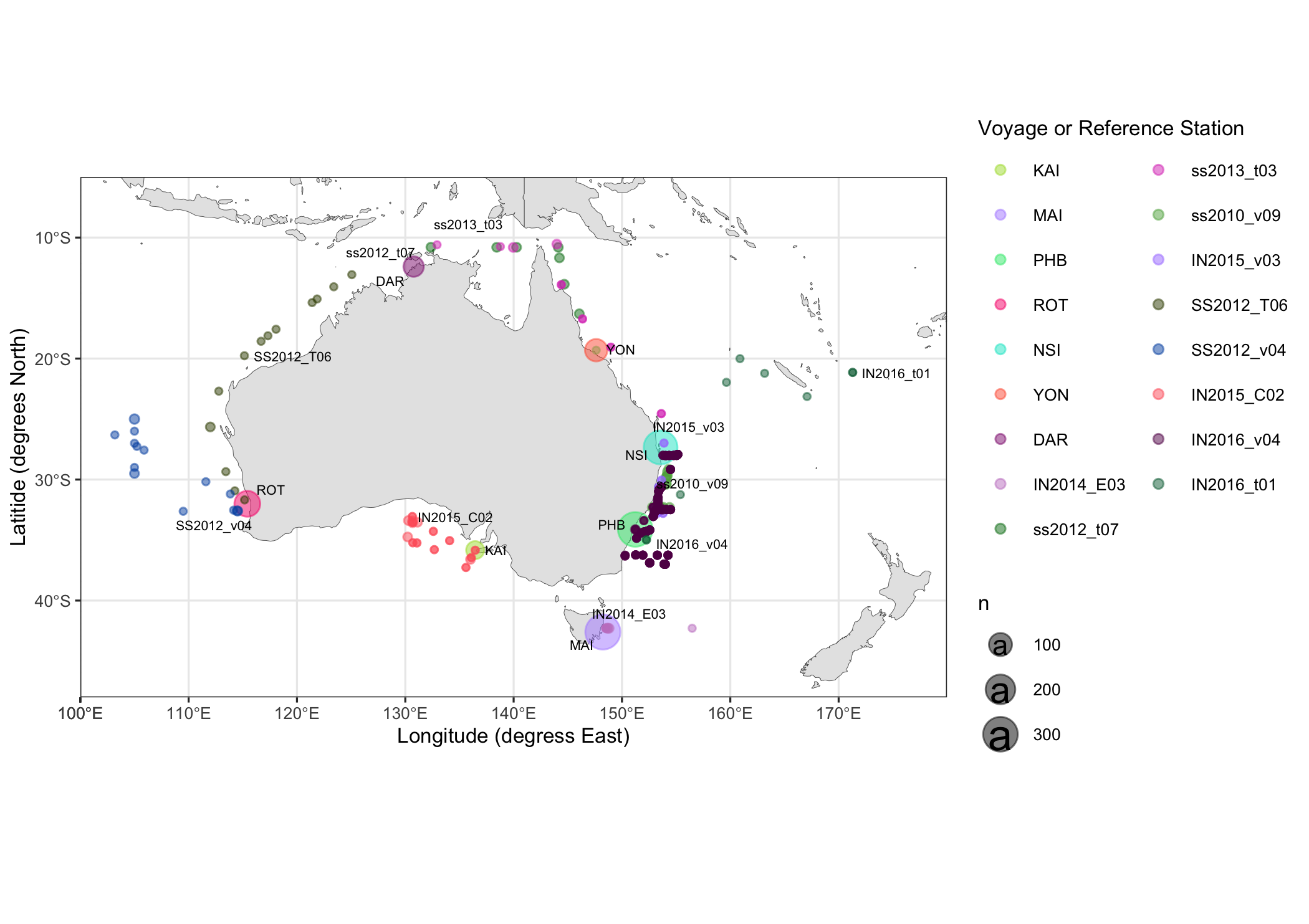
3. Now, a view of where-from and when all of these samples were collected.

world <- ne_countries(scale = "medium", returnclass = "sf")
class(world)

ggplot() +  
  geom_sf(data = world, lwd=0.1) + 
  coord_sf(xlim = c(100, 180), ylim=c(-48,-5))+ 
  theme_bw(base_size=8) + 
  guides(color=guide_legend( ncol=2)) +
  geom_count(data=contextual.long, aes(x=longitude_decimal_degrees, y=latitude_decimal_degrees, color=nrs_location_code_voyage_code), alpha=0.5)+
  labs(y='Latitide (degrees North)', x='Longitude (degress East)') +
  scale_color_manual(values=sitecols, name="Voyage or Reference Station")+
  geom_text_repel(nudge_x = 0.05, data=sites, (aes(x=longitude_decimal_degrees, y=latitude_decimal_degrees, label=nrs_location_code_voyage_code, size=9)))+
   scale_y_continuous(expand=c(0,0), limits=c(-48,-5)) + scale_x_continuous(expand = c(0,0), limits=c(90,180)) 

ggsave('~/AMMBI_MM_samplemap.png', width=7)

contextual.long$type <-contextual.long$nrs_location_code_voyage_code
contextual.long$type<-fct_expand(contextual.long$type, "voyage")

contextual.long$type[!contextual.long$type %in% c("KAI","MAI","PHB","ROT","NSI","YON","DAR")]<- "voyage"
contextual.long$type<-factor(contextual.long$type, levels=c("KAI","MAI","PHB","ROT","NSI","YON","DAR", "voyage"))


ggplot() +  
  theme_bw(base_size=8) + 
  guides(color=guide_legend( ncol=2)) +
  geom_point(data=contextual.long %>% filter(!is.na(date_sampled), depth_m < 100), 
             aes(x=date_sampled, y=round(depth_m/20,0)*20, color=nrs_location_code_voyage_code))+
  labs(y='Depth (m)', x='Date Sampled', title="Timeline of Sampling") +
  scale_color_manual(values=sitecols, name="Voyage or Reference Station")+
  facet_grid(type ~ ., scales='free', space='free') +
  geom_text_repel(nudge_x = 0.1, data=sites, aes(x=date_sampled, y=100, label=nrs_location_code_voyage_code, size=0.5))+
  theme(strip.text.y = element_text(angle = 0)) + scale_y_reverse()

ggsave('~/Timeline_of_sampling.png', width=10)

That is a lot of samples. How many in total?

5. How does the physical and chemical conditions differ between sites and vary over time?

To expore the data in different dimensions we can begin by plotting the relationships between nutrients, temperature, depth and time of year.

ggplot(contextual.long %>% filter(depth_m < 100)) + 
  geom_point(aes(x=jitter(depth_m), y =Temp_C, color=nrs_location_code_voyage_code, size=nitrate_nitrite_μmol_per_l/phosphate_μmol_per_l), alpha=0.5) +
  scale_color_manual(values=sitecols, name="NRS or voyage") +
  theme_bw() + 
  guides(color=guide_legend( ncol=2, override.aes = list(size=7))) + 
  coord_flip() + 
  scale_x_reverse() +
  labs(x= 'Depth (m)',y='Temp (˚C)', title="N:P ratios depicted in a bubble plot")

ggplot(contextual.long %>% filter(depth_m < 100)) + 
  geom_point(aes(x=nitrate_nitrite_μmol_per_l, y =Temp_C, color=nrs_location_code_voyage_code, size=phosphate_μmol_per_l), alpha=0.5) +
  scale_color_manual(values=sitecols, name="NRS or voyage") +
  theme_bw() + 
  guides(color=guide_legend( ncol=2, override.aes = list(size=7))) + 
  coord_flip() + 
  labs(x= 'NO3+NO2', y='Temp (˚C)', title="Nitrate + Nitrite concentrations v. Temp (˚C)")

ggplot(contextual.long %>% 
         filter (!is.na(Temp_C), type!="voyage"),
         aes(x=date_sampled, color=depth_m, y=Temp_C)) + 
          facet_grid (type ~ ., scales='free') + 
          theme_bw() + 
          labs(x="Date Sampled", y="Temperature Range (˚C)") +
          geom_jitter(alpha=0.7, position=position_jitter(w=0.4,h=0.2)) + 
          scale_color_gradientn(colors=oceColorsDensity(100)) +
          theme(strip.text.y = element_text(angle = 0))

marinemicrobes